Function Transformations
We may linearly transform any function by multiplying and adding coefficients to the function’s input and output to create a new function. Say f(x) is our function, then we can create a new function, possibly called g(x), by doing the following:
g(x) = a f(b(x – h)) + k
Where a and k act on the output of f(b(x – h))
and b and h act on the input going into f(x).
Using the diagram, the input or x values control the horizontal positioning of the function’s points. The output, f(x), or y values affect the vertical positioning of the function’s points.
Click the button above to run the Transformations web app. There are considerable supporting information and another button to run the app below.
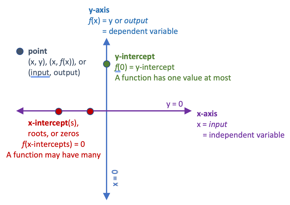
The diagram above is a reminder that a graph’s x-axis represents the input values to the function, and the y-axis represents the values output by the function. Multiplying and adding to a function’s input affects its horizontal position, and multiplying and adding to the output affects the function’s vertical position.
Importance of Transforming Functions
Usually, the function being transformed has the simplest possible form, and all of the transformed functions retain many of the original function’s features. Consider f(x) = x, where the output equals the input. An important feature of this function is that the slope is constant across the entire domain. All of the functions created by multiplying and adding constants to x retain this feature: they all have a constant slope, and they are referred to as linear functions, which we often show as:
y = mx + b
Where m = slope, b = y-intercept, and y = f(x).
For our original function, f(x) = x, this would mean its slope = 1 and the y-intercept = 0.
Many pairs of variables in our world are proportional to each other, and we use linear functions to calculate their numerical relationship. Try building a house, especially the stairs or a slanting roof, without using a linear function!
Another simple function, f(x) = x², is transformed into quadratic functions. You can’t study the motion of objects through the air without the quadratic function!
Features of a Graph of a Function
Graphs of functions allow us to see patterns and features that help identify the function’s basic nature and what makes it unique. To help see them, keep changing your perspective while viewing the graph. First, envision the function without the axes present: describe its shape based on slopes, local/global maximums and minimums, and asymptotes. Horizontal asymptotes are lines parallel to the x-axis that the graph of the function approaches as x tends to ±∞ (infinity). Vertical asymptotes are lines perpendicular to the x-axis near which the function grows without bound (the output goes to ±∞).
Next, view the function relative to the axes. Now size or scale (domain and range), position (x-intercepts and y-intercept), orientation, and symmetry are identifiable.
When possible, write and draw on the graph. Handwritten words help anchor the meaning of the features you are seeing, and drawing helps you slow down your observing process while also noticing the graphs’ spatial relationships.
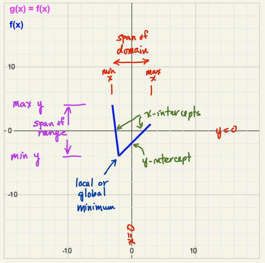
Above are labeled features of a graphed function. Study how each change during different types of transformations.
Also, take note of the slope of the function at different x values. There are two segments with a constant slope in this graph, but one is negative, and one is positive. The magnitude of the two slopes are different, with the left segment having a steeper slope.
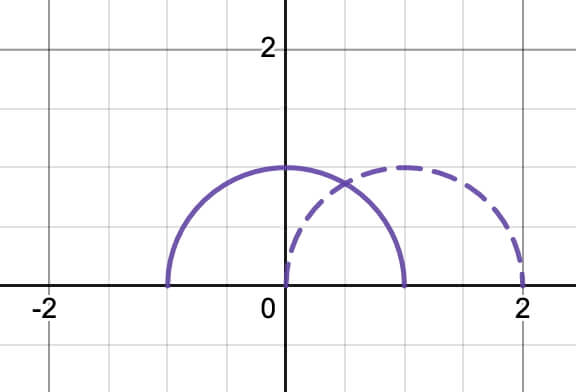
The graph of a half-circle with a radius of 1 is transformed with an h value of +1.
Go to the Desmos activity to explore how functions are transformed as a, b, h, and k change. You may change the function to any that intrigue you.
Patterns of Behavior While Transforming Functions
The web app, Transformations, allows you to create a function, f(x), with a limited domain and range and then change a, b, h, and k to explore how g(x) = a f(b(x – h)) + k is affected.
Identify patterns that are consistent between different starting functions, and try to determine why you are surprised by any outliers. Below are several example cases created with the app. Patterns are available by clicking the dark green toggle button labeled Patterns.
Challenge yourself! Use the web app and/or the animations that follow to see how many patterns you identify on your own. Then compare your list with the ones shown in the toggle buttons.
Click the button above to run the Transformations web app.
The Transformations web app has 9 activities:
1. Create a random function, f(x), and change the a, b, h, and k values to create g(x).
2-4: Based on the graphs of f(x) and g(x), identify which one, two, or three of the four coefficients create(s) g(x) from f(x).
5: Use the randomly generated scenarios to quiz yourself to identify which of the four coefficients are creating g(x).
6-9: are similar to 2-5 except now you must identify the values of a, b, h, and k.
For the two quizzes, earn a personalized certificate of accomplishment with a minimum score of 4 correct answers in 5 tries.
Acknowledgments
I want to thank my teaching colleagues Mark Engerman and George Larivee, for inspiring the web app’s creation and improvements.
Changing a
Using these animations, create a list of how a function transforms as the coefficient a changes from 3 to -3 in 0.25 increments.
Recall that a is multiplying the output of the original function.
Patterns
- a > 1 vertically stretches g(x)
- 0 < a < 1 vertically compresses g(x)
- a = 0 creates a horizontal line.
- a < 0 flips g(x) across the x-axis.
- -1 < a < 0 vertically compresses g(x)
- a < -1 vertically stretches g(x)
- The shape of the function changes since slopes change as g(x) is vertically stretched or compressed
- The x-intercepts remain the same for f(x) and g(x) since these represent output values of zero and a * 0 = 0.
- The maximum and minimum values of the range change based on how far they are from the x-axis (y = 0)
- The range of output values changes such that the span of g(x) range = a * span f(x)’s range.
- The x values for f(x) and g(x) remain unchanged as a changes, so the domains of both are identical too.
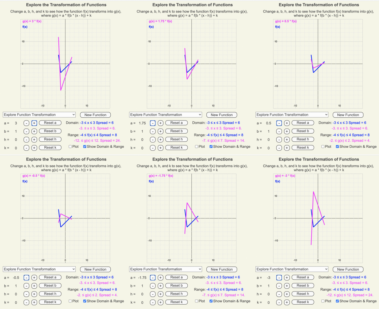
Animation of how g(x) (magenta line) changes as the output of f(x) (blue line) is multiplied by a as it changes from 3 to -3 in increments of 0.25.
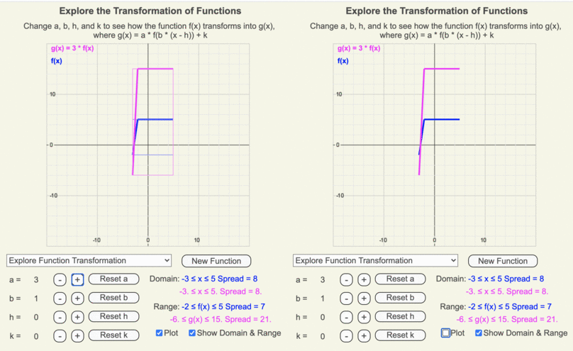
Animation of how the domain and range of g(x) (shown by the thin magenta box) differ from those of the original function f(x) (shown by the thin blue box) when a = 3.
Changing b
Using these animations, create a list of how a function transforms as the coefficient b changes from 3 to -3 in 0.25 increments.
Recall that b is multiplying the input going into the original function.
Patterns
- b > 1 horizontally compresses g(x)
- 0 < b < 1 horizontally stretches g(x)
- The transformation when b = 0 does not exist.
- b < 0 flips g(x) across the y-axis.
- -1 < b < 0 horizontally stretches g(x)
- b < -1 horizontally compresses g(x)
- The shape of the function changes since slopes change as g(x) is horizontally stretched or compressed
- The y-intercept remain the same for f(x) and g(x) since this represents an input value of zero and b * 0 = 0.
- The maximum and minimum values of the domain change based on how far they are from the y-axis (x = 0)
- The domain changes such that the span of g(x)’s domain = span of f(x)’s domain / b.
- The y values for f(x) and g(x) remain unchanged as b changes, so the ranges of both are identical too.
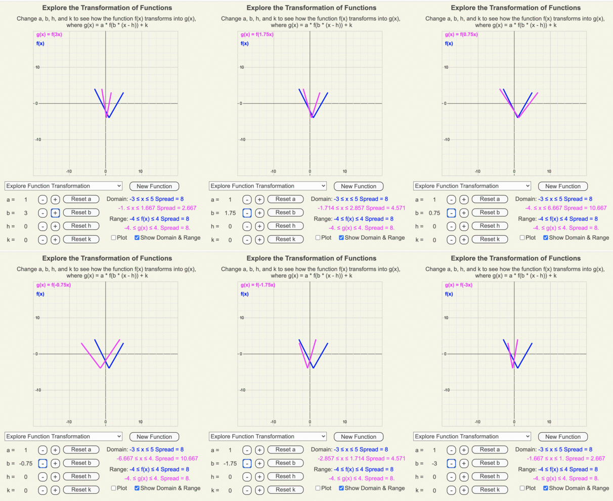
Animation of how g(x) (magenta line) changes as the input going into f(x) (blue line) is multiplied by b as it changes from 3 to -3 in increments of 0.25.
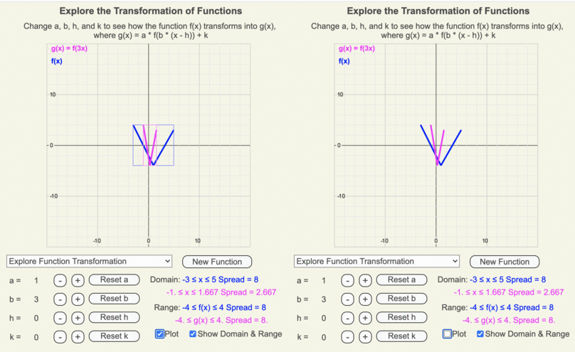
Animation of how the domain and range of g(x) (shown by the thin magenta box) differ from those of the original function f(x) (shown by the thin blue box) when b = 3.
Changing h
Using these animations, create a list of how a function transforms as the coefficient h changes from 5 to -5 in unit increments.
Recall that h is added to the input of the original function.
Patterns
- When h > 0, g(x) moves to the right of f(x) by h units.
- When h < 0, g(x) moves to the left of f(x) by h units.
- The shape of the function remains constant as h changes.
- The x-intercepts of g(x) shift from f(x) by an amount of h.
- The maximum and minimum values of the domain shift from f(x) by an amount of h.
- The span of g(x)’s domain = span of f(x)’s domain.
- The y values for f(x) and g(x) remain unchanged as h changes, so the ranges of both are identical too.
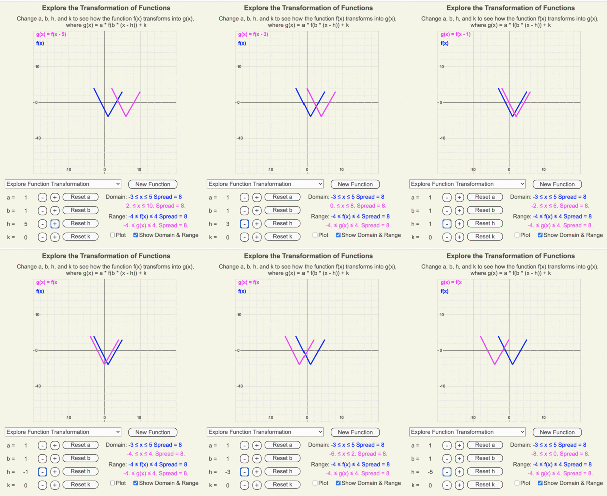
Animation of how g(x) (magenta line) transforms from f(x) (blue line) as h changes from 5 to -5 in increments of 1.
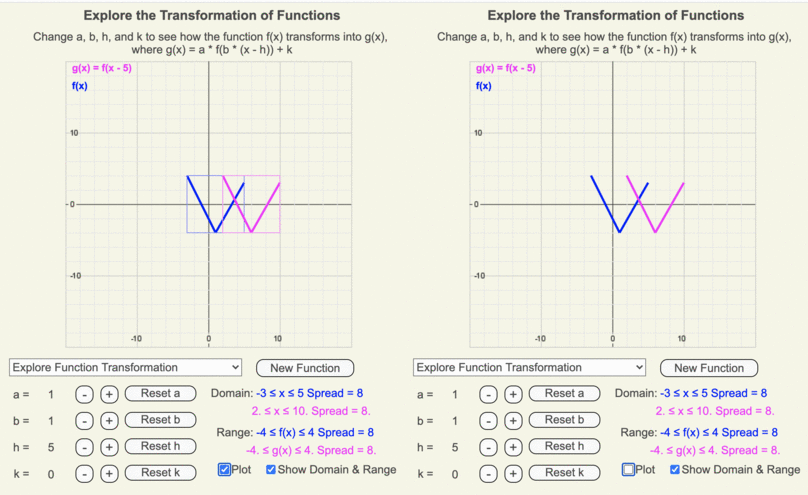
Animation of how the domain and range of g(x) (shown by the thin magenta box) differ from those of the original function f(x) (shown by the thin blue box) when h = 5.
Changing k
Using these animations, create a list of how a function transforms as the coefficient k changes from 5 to -5 in unit increments.
Recall that k is added to the output of the original function.
Patterns
- When k > 0, g(x) moves up k units from f(x).
- When k < 0, g(x) moves down k units from f(x).
- The shape of the function remains constant as k changes.
- The y-intercept of g(x) shifts from f(x) by an amount of k.
- The maximum and minimum values of the range shift from f(x) by an amount of k.
- The span of g(x)’s range = span of f(x)’s range.
- The x values for f(x) and g(x) remain unchanged as h changes, so the domains of both are identical too.
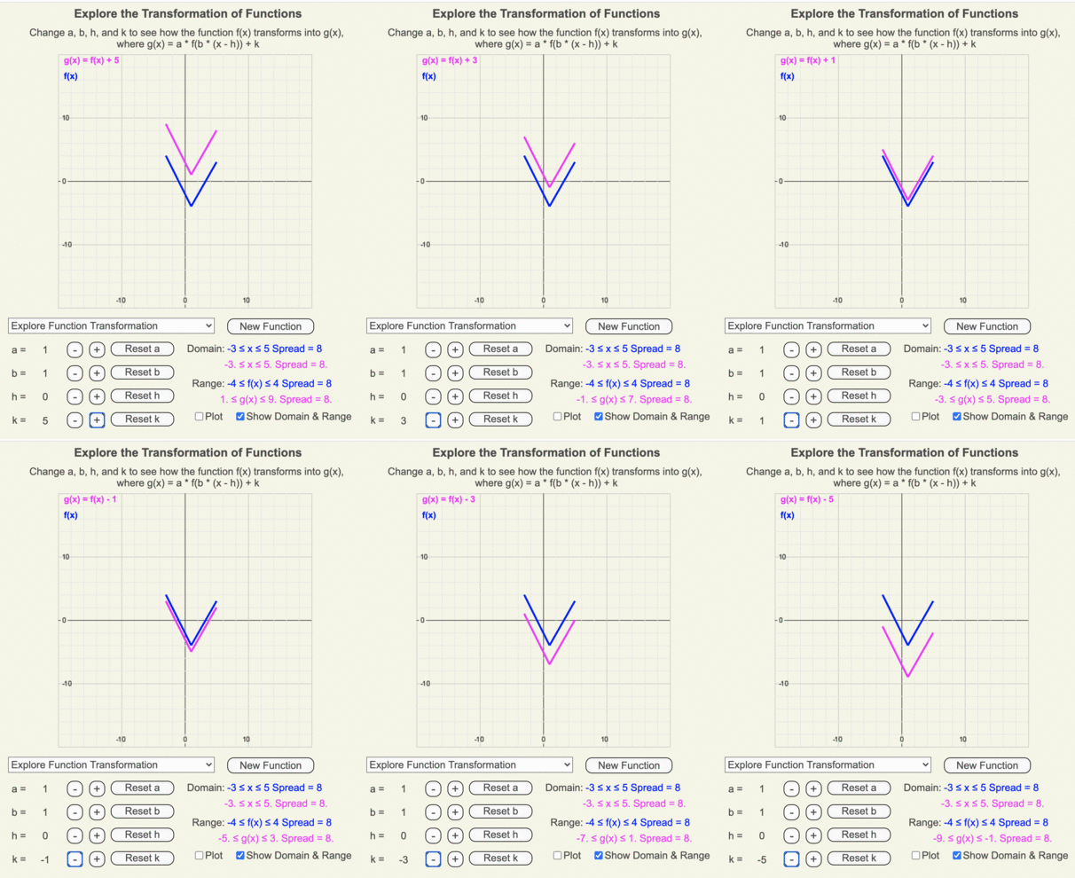
Animation of how g(x) (magenta line) transforms from f(x) (blue line) as k changes from 5 to -5 in increments of 1.
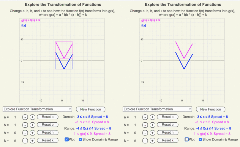
Animation of how the domain and range of g(x) (shown by the thin magenta box) differ from those of the original function f(x) (shown by the thin blue box) when k = 5.
Conceptually Understanding Function Transformations
Once you’ve completed a mathematical calculation, you hope your answer is correct, but how do you know for sure? The first step in checking your work is asking whether the results fit within your understanding of the function’s expected behavior. Understanding how functions transform will help identify the fewest pairs of inputs and outputs needed to check your work’s accuracy thoroughly.
When working with data, graphs, or functions, there are many opportunities to make mistakes, leading to incorrect results:
- Was the input data typed correctly?
- Were the math manipulations done properly?
- Was the formula mistyped into the computer program or spreadsheet?
It is so easy to miss a small error in a stack of numbers, math symbols, or computer code, so an excellent way to check your work is to find key numbers to test in your accuracy. Conceptually understanding how a basic function is transformed will help identify input and output values that will quickly verify your work’s accuracy.
Develop Your Conceptual Understanding
The web app above, Transformations, has four activities to help you identify the coefficients involved in transforming a function, not actually calculate their values. These activities are intended to support looking for patterns and clues and develop your conceptual understanding of function transformations, which are useful when you are tasked with calculating the coefficients.
Calculating Function Transformations
There are two general scenarios in which you calculate function transformations:
- You are given the starting function in graph or data form and the values of a, b, h, and k to calculate the transformed function, or
- You are given the two functions in the form of data or graphs, and you need to calculate a, b, h, and k.
Scenario 1: Convert (x, y) points of the starting function, f(x) to those of the transformed function, g(x):
xg = xf / b + h
yg = a * yf + k
Remember to multiply and divide before adding or subtracting!
As a check, did g(x) stretch/compress and shift in the vertical and horizontal as expected? This is where your conceptual understanding comes in handy!
Resources
Lumen Learning provides well-illustrated and highly interactive materials to understand and calculate function transformations.
Practice Problem: Given graph of f(x), draw -3 f(-0.5(x + 5)) – 5
Step 1: Identify a, b, h, and k from the transformation formula and envision the final result.
Since the convention of the transformation formula is
a(f(b(x – h)) + k
then
-3 f(-0.5(x + 5)) – 5
means
a = -3
b = -0.5
h = -5 (Notice: x – (-5) = x + 5)
k = -5
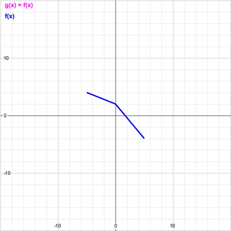
Above is the graph of f(x), which is to be transformed in this example problem.
Step 2: Identify key points to transform.
In this case, since f(x) consists of two connected linear segments, find the points of the endpoints of each segment. Since the transformed function will also have two connected linear segments (unless a = 0, which would create a horizontal line), there are only three points to identify on f(x) that will also define g(x).
From left to right, the three points are:
| (-5, 4) |
| (0, 2) |
| (5, -4) |
Since every fifth line represents 10 units, the grid lines are 2 units apart.
Now you have two choices:
- Work numerically to transform the points and then plot, or
- Work graphically and numerically at the same time.
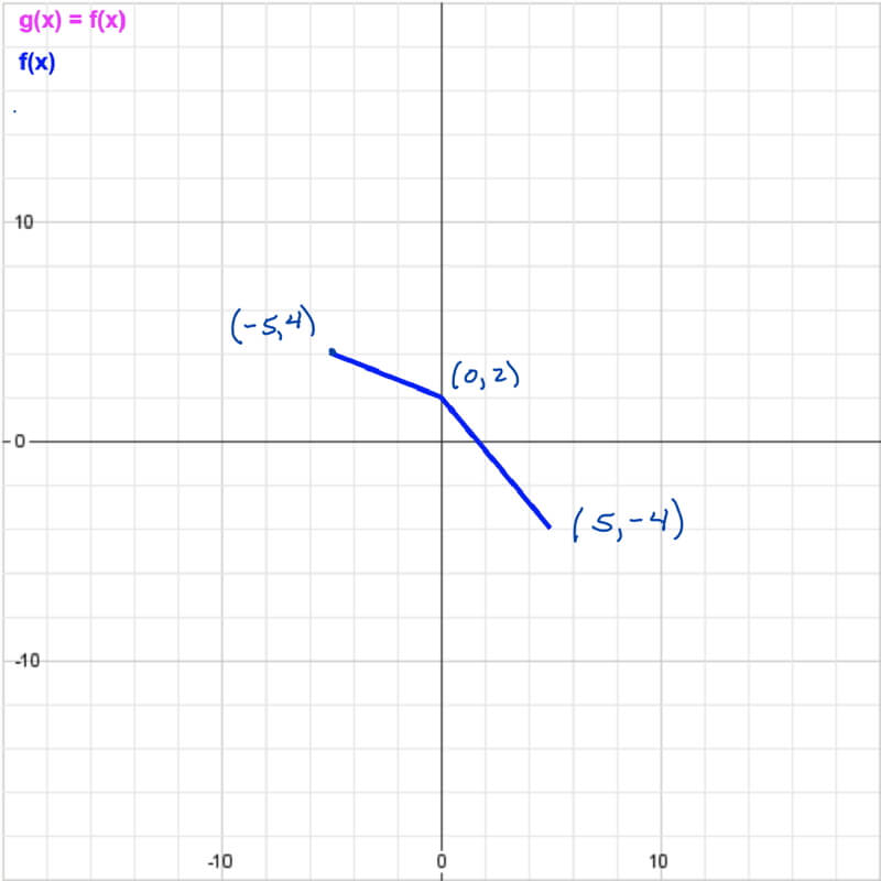
To identify the coordinates of the points, since every fifth line represents 10 units, the grid lines are 2 units apart.
Option 1: Transforming Numerically
Remember:
xg = xf / b + h
yg = a * yf + k
and to multiply and divide before adding or subtracting!
|
Original Points |
Apply b: x / -0.5 |
Apply h: New x – 5 |
Apply a: y * (-3) |
Apply k: New y – 5 |
| (-5, 4) | (10, 4) | (5, 4) | (5, -12) | (5, -17) |
| (0, 2) | (0, 2) | (-5, 2) | (-5, -6) | (-5, -11) |
| (5, -4) | (-10, -4) | (-15, -4) | (-15, 12) | (-15, 7) |
Once the calculations are done, plot the points. In the table above, these would be the points in the right-most column.
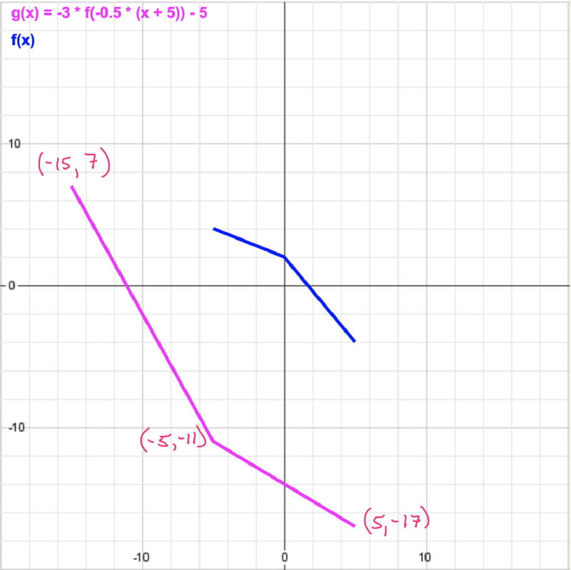
The magenta line represents the transformed example problem.
Option 2: Transforming Graphically & Numerically
Rather than manipulate the numbers in a table, as shown above, you may work directly on the graph, but you still need to apply the transformation coefficients using these equations:
xg = xf / b + h
yg = a * yf + k
Remember to multiply and divide before adding or subtracting!
Once the calculations are done, connect the final points on the graph.
Working on the graph becomes busy when dealing with three or more transformation coefficients, but it may be done, especially if you use color pencils.
Visual Check of Your Answer
If there are asymmetries or special features in your function, check to see if their position in the transformed function agrees with what you identified should have happened in Step 1.
In our example problem, the shortest segment of the two is in the upper left part of the function of our original function, and after a flips f(x) over the x-axis, and b flips it over the y-axis, the shortest segment should be on the lower right of the transformed function. And it is!
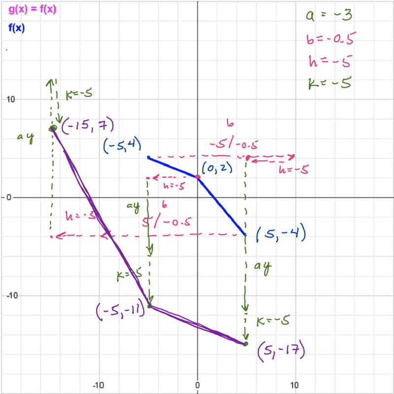
The magenta dashed lines represent the effects of the function’s x-coordinates by applying b and h coefficients (calculated first in this example). The green dashed lines show the effects of applying a and k coefficients to the y-coordinates (calculated second). The purple line represents the transformed example problem.
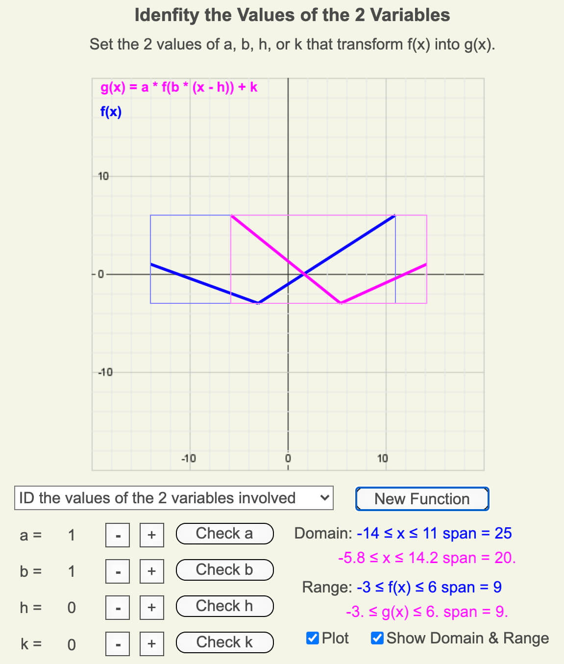
Scenario 2: Given graphs and data, calculate a, b, h, and k
- Since the two graphs have identical ranges, a = 1 and k = 0.
- g(x) is flipped across the y-axis, so b < 1.
- 1/|b| = domain span of g(x) / domain span of f(x) or
- |b| = domain span of f(x) / domain span of g(x) = 25 / 20 = 1.25
- Combining Steps 2 and 4, b = -1.25.
- Remove the horizontal compression from the domain values of f(x) – remember that a negative value of b causes a maximum domain value to become a minimum domain value and vice versa:
- min x = 11 / b = 11 / (-1.25) = -8.8 and
- max x = -14 / (-1.25) = 11.2
- Compare these uncompressed domain values of f(x) to g(x) to calculate h:
- h = 14.2 – 11.2 = -5.8 – (-8.8) = 3 (This is a good check, both function’s maximum and minimum domain values must shift by the value of h.)
Check: b = -1.25 and h = 3 so g(x) is flipped across the y-axis and compressed horizontally and shifted to the right by 3.
As you can see, this is a many step process that involves:
- information from the graph of the function,
- data gleaned from the graph, and
- an understanding of the form of the function transformation.
No one form provides all of the information; rather, working with each is required to gather the clues and apply them in the proper order.
Topics in Observing
- Our Senses and Brain
- Perspective,
- Technology,
- Measurement,
- Data, Graphs, and Functions
- Function Transformations
- Contouring, and
- Improving Observational Skills.
Measure your:

0 Comments