
Math Modeling
Modeling provides insights into real-world situations. Models can be physical, but they can also be built with math. A mathematical model describes a system, process, or event using mathematical concepts and methods. Models built on math help us better understand, explain, and predict the responses of the interconnected components over time or space, which is why they are essential tools for scientists, engineers, mathematicians, economists, financial analysts, business people, musicians, linguists, philosophers, and even athletes. Despite the widespread use of models, remember they are tools, and all tools have limitations. Just like data, there are no perfect tools. Even with machine learning, there will always be room for improvement.

A concept map illustrating the major steps of creating, developing, and improving a math model of a real world system, process, or event.
Goals and Syllabus for Math Modeling Course
Goals for Math Modeling Course
Jodi Pickle Spring, 2023
- Introduce a variety of types of math models and their applications by using & modifying existing math models
- Provide opportunities to explore your interests, applications, & understanding of math by creating your math models
- Provide opportunities to go beyond your initial successes & learn from setbacks
- Provide opportunities to revisit your model to improve, modify, & expand
Grading
- Homework/Challenges – 20%: Homework will be graded based on your process of solving the problem and how you checked your work. There will be roughly 2.5-3 hours of work outside of class each week (~ 1 hour following each class).
- Notebook – 20% — Document your daily progress, ideas, mathematical calculations & manipulations, and results & findings during your projects, homework, and challenges. Bring your notebook (digital or paper) to class so I may review & provide comments/suggestions.
- Project 1 – 20% — Create, test, document, beta test with others, and deliver a mathematical model involving a topic that interests you.
- Concept Map: 5%
- Weekly Presentation on Progress: 5%
- Instructions to Use Model & Findings from Using Model: 5%
- Quality of Model: 5%: accuracy, interface, and visualizations
- Project 2 – 20% — Create, test, document, beta test with others, and deliver a mathematical model involving a topic that interests you. You may build on Project 1 if you like, or create a new model that interests you.
- Concept Map: 5%
- Weekly Presentation on Progress: 5%
- Instructions to Use Model & Findings from Using Model: 5%
- Quality of Model: 5%: accuracy, interface, and visualizations
- Final Presentation – 10%
- Assessment of the Risk You Took During the Semester – 10%: Based on your comfort level and experience with math, how far did you venture outside your existing abilities that you brought to the course? Due on the day of the final exam.
What is Math?
In Jo Boaler’s book, Mathematical Mindsets, she defines math as the study of patterns. Think about a world without patterns. Every process on the planet would be random. There would be no predictability; survival would be a roll of the dice every second of every day. If this were so, and if life existed on this “random” planet, it would be very simplistic with a very short life span. All living organisms on Earth survive and thrive because they recognize and adapt to patterns.
Based on this, most math used in math modeling tends to be based on functions since every input is mapped on a unique output. Equations can be used; however, they are a bit more complex since they require limiting the output to one of the possible outcomes for the given input. Think of the equation of a circle. All except four points of the circle have two outputs for a given input.

Explore the behavior of a function by adding and multiplying values to the input and output of an existing function. Click on the graph to go to the activity created on Desmos. For more insights into this activity, see Function Transformations.

A graph of a circle with a radius of 2 and the center point (0, 0). Explore how the circle changes by changing the equation of the circle by clicking on the graph to go to the activity created on Desmos.
Model without Math First
First, solve the puzzle, on the right. Work by yourself or with a peer. List the rules that you create in the edges of your puzzle as you go along.
Second, make a puzzle on your own using two copies of the blank puzzle template. Why two? First you must create the solution and use this to create the puzzle to be solved using the second. Bring your new puzzle to class for someone to solve.
Finally, make a list of questions and insights you gained about the the nature of and solving the puzzle as you created and tested your puzzle. These reflections show how modeling changes our perspective on a topic being studied so we can deepen our understanding. The process of creating a model provides many opportunities to explore the procedure(s) you are modeling.

Solve this puzzle. Click on the image to download a pdf to print, or recreate by hand on a blank sheet of paper.

Click on the image to download a pdf for making your own puzzle.
A few questions to get you started as you create a new puzzle
- What is the fewest number of points needed, so your puzzle has one solution?
- To answer this, work from both ends of the problem.
- a) If you have one point, would there be more than one solution?
- b) If you provide 80 points, how many solutions are possible?
- How do you know your model is solvable?
- How difficult is your puzzle to solve?
- Can I include numbers that aren’t along the edges?
- If you try placing numbers anywhere within the grid, does it change the feel of the original game?
Tangent Activity: Can You Complete the Hamilton Path?
In order to guarantee that your puzzle above has a solution (but it may not be solvable or have only one solution depending on how many clues you give), you are drawing a Hamilton Path. When I first started doing these puzzles, I likened my efforts to trying to draw a “number snake,” however, one of my students shared that it was actually a Hamilton Path which is a path that goes through each vertex of a graph exactly once, and in this case, the vertices are defined by the centers of the 81 squares.
But something interesting arose when people started drawing the solutions – they didn’t always work(!). So, the challenge is, what pattern do you notice depending on where you place the start of your Hamilton Path (or where do you place “1”)?
Suggestion: Print out four blank grids to attempt to draw each Hamilton Path.

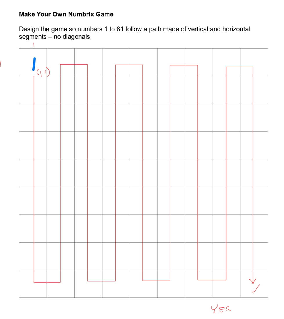
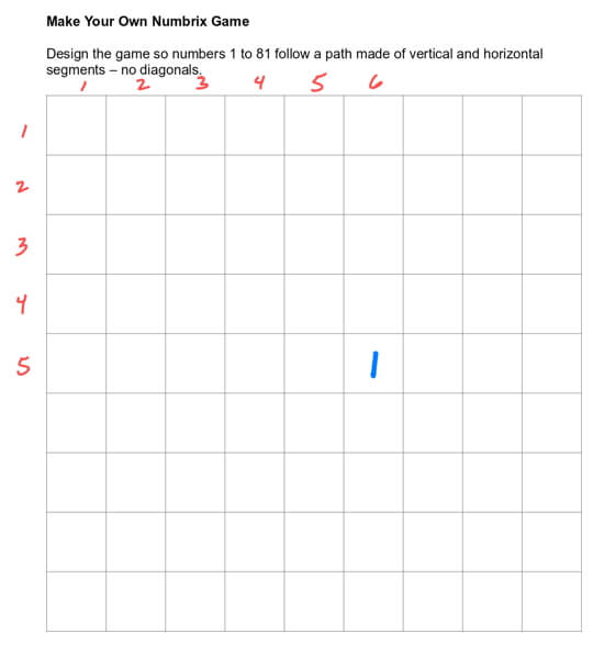
Can you create a Hamilton Path when you place 1 (the starting point) in this square?
Answer

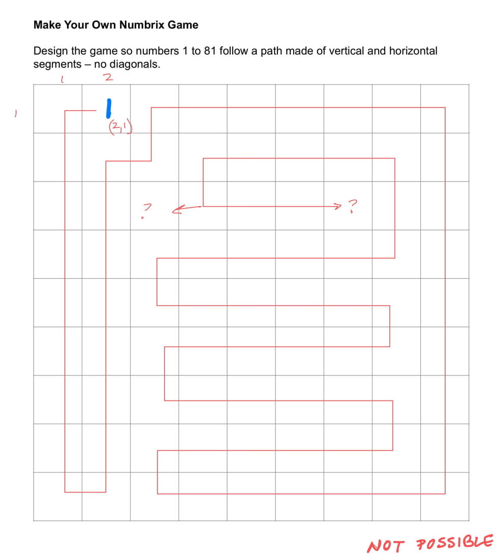
Can you create a Hamilton Path when you place 1 (the starting point) in this square?
Answer

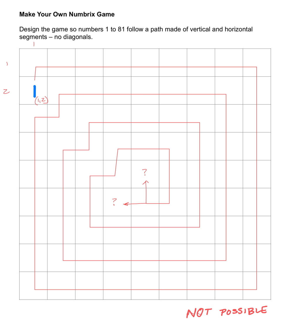
Can you create a Hamilton Path when you place 1 (the starting point) in this square?
Answer

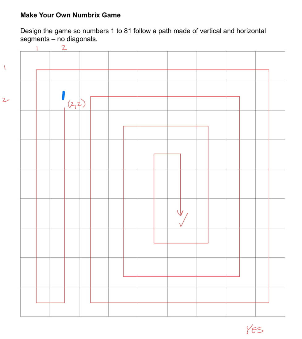
Can you create a Hamilton Path when you place 1 (the starting point) in this square?
Answer
")
Based on the patterns observed in the four cases, predict whether you can create a Hamilton Path when the 1 (starting point) is placed in this location.
Answer
The pattern seen in the four puzzles with the starting points (1,1), (2,1), (1,2), and (2,2) suggest that when the starting points are both even or both odd, a Hamilton path may be drawn. If the coordinates are mixed, one even and one odd, then a Hamilton path is not possible. Since the challenge puzzle has a starting point at (6,5), where one is even and one is odd, is not possible.
The patterns should also hold for the ending points of the Hamilton puzzle. Use these patterns to help you solve the puzzles!
More experiments on starting points
To explore complex ideas, try to map decrease the complexity. Rather than use 9×9 grids, to make it faster, let’s try a 3×3 grid to explore the patterns.
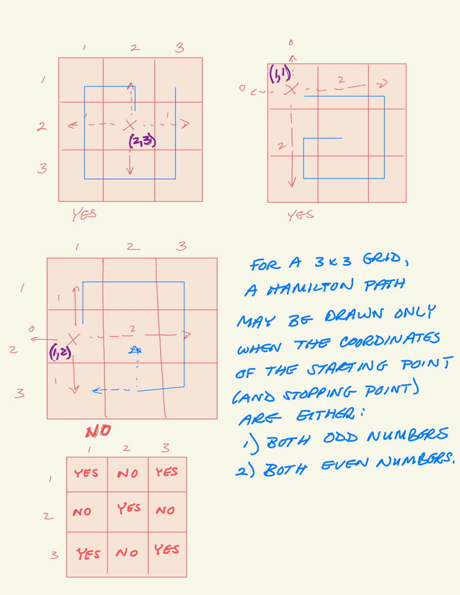
This supports what we saw with the four cases above.
Tangent Activity 2: What about an 8×8 Grid?
If you have an 8×8 grid of squares, does it matter where you start your Hamilton Path? Create your experiments to find out.
Experiments on even by even grids
Rather than use 8×8 grids, to make it faster, let’s try a 4×4 grid to explore the patterns.
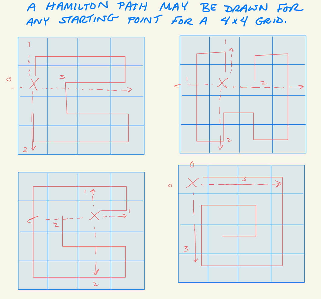
This suggests that drawing Hamilton paths for even by even grids do not have any restrictions on where you start (or end) the puzzle.
Experiments on even by odd grids
Let’s try a 4×3 grid to explore the patterns.
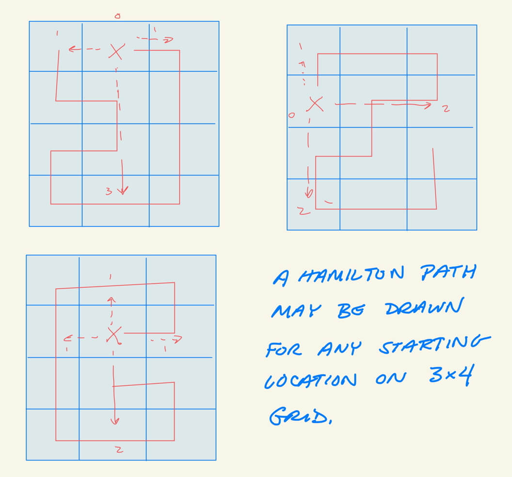
This suggests that drawing Hamilton paths for even by odd or odd by even grids do not have any restrictions on where you start (or end) the puzzle.
Flow of Math Modeling
My calculus course in the late 1970s required programming various algorithms to help us explore concepts from a new perspective. That summer, I worked for a professor working with a program to study evolution by studying the morphology of bivalve shells. Both of these experiences changed my approach to math. The independent exploration of concepts I was learning and applying these to my own ideas resonated with me deeply.
This course is designed to use free software (CmapTools, Desmos, Google Sheets, StarLogo, and NetLogo) to explore math models.
The general flow to learning how to work with models in each of these platforms is to:
- use existing models,
- modify them, and
- create math models of my student’s ideas and interests.
Concept Mapping Activity
When you create your own math models, you will concept map to help users visualize how the components interact in your model. To learn how to create a concept map, start with concept mapping some of the components that make up you.
One way to think about a concept map is that each concept is a noun and the works linking the concepts is an action verb.
Start by creating a list of nouns that describe you. Don’t worry about the order, just record them in what is called a parking lot.
Once you have a list you feel is complete, group your nouns in related clusters. Enter these on CmapTools, and use the linking tool to create arrows and add the action verbs.
Share your concept map with a peer, let them spend a minute or two reviewing it, and then let them explore your life with you. Concept maps are surprisingly easy to read and comprehend.

A concept map of a number of my interests and activities that have meant quite a bit to me. For more help on concept mapping, see Matti’s concept mapping tutorial.
A Word About Tangents, Creativity, and Math Modeling
A tangent to a curve is a line that touches a single point on the curve. Keeping to the general spirit of this definition, a tangent thought touches an idea (or two…) but then goes off in new directions you may not have thought about. Talk to any creative person; I am sure their tangent thoughts regularly inspire them. Creativity needs to take nuggets of our knowledge to new places in our imagination.
In working with math models, you will have many opportunities to ask, “What happens if…?” And these are jumping-off places to explore tangent thoughts and ideas. If the model has ways to change inputs, use them. If you can modify the model’s math, then you may try more powerful ideas. And sometimes, you will want to create a new model based on some of the discoveries you made from existing models, but they were too limited to test your ideas. Explore tangent thoughts by using, modifying, and creating math models.

Above is the tangent line (black) to the point (1,1) for the function y = x² (red).