Shooting a Basketball Activity
What does it take to make a free throw in basketball? Pro players may make it look easy, but it takes a lot of practice to develop one’s skill.
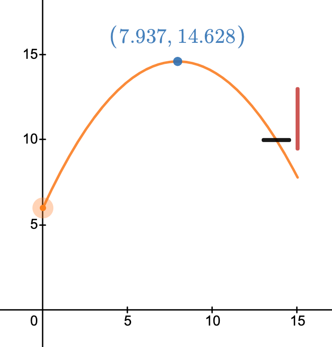
Open the basic model created in Desmos (click on the image on the right) and explore how to make a free throw by changing the three variables:
- The height (h) of the ball when released from the shooter’s hand,
- The angle (θ) of the ball as it leaves the shooter’s hand, and
- The ball’s velocity (v) at the moment of release.
One way to mathematically model the ball moving through the air is to break it into horizontal (x) and vertical (y) components since the ball only accelerates vertically downward due to gravity.
In the horizontal, if we are standing where we will begin to measure the distance the ball moves (so the zero position):
x = v(horizontal) t
where t = time the ball has left the shooter’s hand.
The ball is not accelerating in the horizontal direction, but it is when we consider the vertical direction.
y = h + v(vertical) t – 0.5 g t²
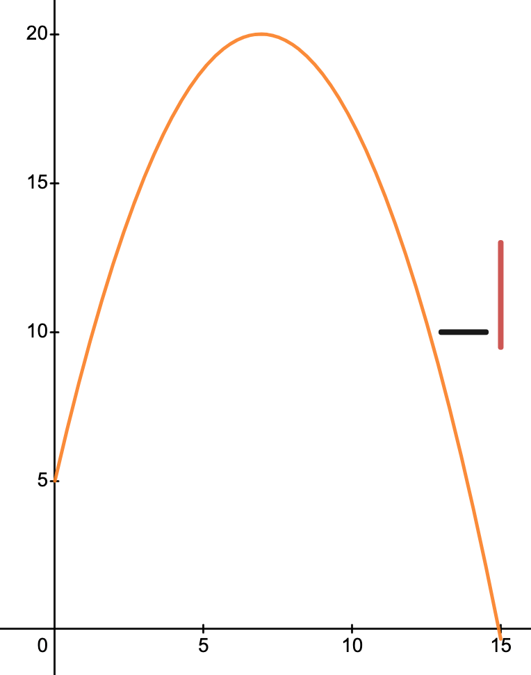
Open the activity by clicking on the graph or click here.
Horizontal and Vertical Velocity
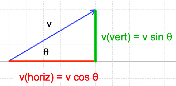
Velocity is a vector, which is a variable that has both magnitude and direction. In this case, the magnitude is the speed of the ball. One of the benefits of using horizontal and vertical motion components is that they are perpendicular to each other. Since we are working with a right triangle, use trigonometric functions, sine and cosine, to calculate the horizontal and vertical velocities (see the diagram on the right).
Combining the two sets of equations creates
x = v t cos θ
y = h + v t sin θ – 0.5 g t²

Use trigonometric functions, sine (sin) and cosine (cos), to break the release velocity into horizontal and vertical components.
Math Manipulation Challenge
The following are activities to modify the existing math model that you need to open at the top of the page.
1) Combine the two equations for vertical and horizontal motion above to create one equation that describes the ball’s trajectory through the air as written in Desmos.
2) What is the velocity in feet per second in miles per hour? Note: 1 mile = 5280 feet.
3) A more challenging problem: If you know the release angle, calculate the ball’s velocity as it leaves the shooter’s hand so that it falls through the center of the basketball rim, 10 feet high and 13.75 feet away from the foul line.
-
- Duplicate the model and add this equation while eliminating the release angle slider. This will provide a visual check that your model is correct.
Radians
Angles are often measured in degrees, where a circle is 360°, but they may also be described in radians. A radian measures an angle based on the radius (r) and the arc length. Since a circle’s circumference is 2πr, which is also 360°, one radian equals 360°/2πr or 57.3°. Many spreadsheets and Desmos use radians, rather than degrees, when calculating sine and cosine values.
For visuals and more information, see Math is Fun.
Answers
1. Desmos efficiently plots functions, so we need a function based on an independent variable: x. We have two equations:
x = v t cos θ and
y = h + v t sin θ – 0.5 g t²
We want to combine them and notice that t is in both equations. Using the first,
t = x / (v cos θ)
Then substitute this into the second equation:
y = h + v sin θ x / (v cos θ) – 0.5 g (x / (v cos θ))²
This simplifies to
y = h + x tan θ – 0.5 g x² / (v cos θ)²
Checking the units: ft = ft + ft – ft² * (ft/s²) / (ft²/s²) = ft + ft + ft² * (ft/s²) * (s²/ft²) = ft + ft + ft It checks!
2. 1 ft / s * mile / 5280 ft * 60 s / min * 60 min / hour = 0.682 miles / hour
So to convert a value in ft / s, multiply it by 0.682 miles/hour per ft/s.
For example, 20 ft/s = 20 * 0.682 mph = 13.6 mph.
3. For this challenge, we know the horizontal distance the ball must travel for a perfect swish: 13.75 ft. Use this with the work done in Challenge 1 above to isolate the launch velocity using values we are provided either from knowing the dimensions of a basketball court or were selected with sliders in Desmos.
What we know:
Distance from the foul line to the rim’s center: 13.75 ft.
Height to the rim: 10 ft.
g (acceleration of gravity) = 32.17 ft/s².
Release angle, θ, is selected with the slider.
Now, the x = v t cos θ becomes 13.75 = v t cos θ 0r t = 13.75 / v cos θ.
Substitute this into y = h + v t sin θ – 0.5 g t² so 10 = v sin θ 13.75 / v cos θ – 0.5 g (13.75 / v cos θ)²
This simplifies to: 10 = h + 13.75 tan θ – 3041.1 / (v² cos²θ)
Isolate for v, which is the release velocity and what you needed to calculate:
v = √(3041.1/(13.75 tan θ + h – 10) cos²θ)
Notice that you could have worked with the equation you arrived at in Challenge 1.
The units check for all of the terms, and, an even better test, when you create your model, the shot trajectory always goes through the center of the basket when you change the release height and angle! If you want to try it out, here is a working version.
Alternate Solution: You don’t need to create one equation that Desmos will plot; instead, calculate a variable used in a formula to simplify it. This can make it easier to enter the formulas since they aren’t as complex (more room for typos and misplaced parentheses when typing one complex formula). You may see if the intermediate calculation is correct since Desmos displays the value.
The more you play with Desmos, the more you will appreciate its flexibility and capabilities!
Math Manipulation Challenges (Part 2)
1) Calculate the position of the ball when it is at its peak height above the ground. Key: at this point, the ball’s vertical velocity is zero while still having the same horizontal velocity as it did when it left the shooter’s hand.
Remember, the ball only accelerates in the vertical direction by a magnitude of g = 32.17 ft/s². There is no acceleration in the horizontal direction.
The definition of acceleration is
a = Δv / Δ t = change in velocity/change in time
Using the vertical direction,
-g = (v(peak) – v sin θ) / (t(peak) – t(initial))
Since v(peak) = 0 and t(initial) = 0, then
– g = -v sin θ / t(peak) or
t(peak) = v sin θ / g
Use this time to calculate the x and y position of the ball at its peak height and plot in your Desmos model.
2) Using the “perfect swish” model you created in the first set of challenges above, find the maximum and minimum velocities so that the ball still goes through the hoop without hitting it (so still a swish).
3) What is the minimum angle needed for the ball to swish through the hoop? Tip: draw out how the ball goes through the hoop.
In Challenges 2 & 3, the circumference of a male basketball is 29.5 inches, and a female ball is 28.5 inches.

An example of the peak ball position for a perfect swished free throw. The ball was 14.628 ft above the court and 7.937 feet away from the shooter when its vertical velocity was zero.
Answers
1. Since the time to reach the peak is now calculated, include the peak time into:
x(peak) = v t(peak) cosθ and
y(peak) = h + v t(peak) sin θ – 0.5 g t(peak)²
Note: In Desmos, t(peak) was calculated as P and used in the two equations above rather than substituting the equation for t(peak) into each equation, simplifying and entering these formulas into Desmos.
2 & 3. As in 1, calculate the time to reach a specific horizontal or vertical position. Tip: Calculate the radius of a male or female basketball using
Circumference = 2 π radius
Here is a model that uses the “perfect swish” calculations in the first set of challenges.
How Do You Know Your Equation is Correct?
Since you will be coming up with your ideas for math models, you can’t rely on having the answers provided or even the teacher acknowledge you are correct. It is up to you to have a variety of ways to check your answers.
Work with your peers to devise various ways to prove your model’s equation(s) is correct. Compare your ideas with the suggestions posted on the right.
Suggestions
- As alluded to in the previous challenge, plot your result to see whether it agrees with what it was expected to do – in this case, the ball will be 13.75 ft away from the shooter and 10 ft off the ground. If it isn’t, you know you made a mistake either in your math manipulation or typing the equation into Desmos.
- Test many conditions to see if the behavior is consistent. For example, if you forget the Desmos requires radians, and you pout in degrees, small changes in an angle create what appears to be erratic behavior. Try this model out to see the behavior for yourself.
- Unit/Dimensional Analysis: Every term in the equation must have the same units (a term is a collection of coefficients and variables being multiplied or divided), and they agree with what you were trying to calculate. For example, in the vertical position equation, identify the units for each term:
- y is in feet,
- h is in feet
- v t sin θ = ft/s * s = ft
- 0.5 g t² = ft/s² * s² = ft
- Note: the sine or cosine of an angle is a unitless number
- The units for each term are the same and agree with what we were trying to calculate.
- If there are example problems with answers, compare your results.
- Use another way to calculate the numbers, such as a calculator. This could be for the entire equation or parts of the equation – remember, you can output parts of the equation in Desmos and the other programs we will use.
- Test the extremes, such as using zero for a variable’s value, and see if the results are what you expect.
For example, if the velocity = 0, then x = 0 sin θ.
If θ = 90º, then x = v cos 90º = v 0 = 0.
WARNING: Check your trig calculations to ensure you are using the correct units for the angle (degrees or radians). In particular, use 90º = π / 2 radians, then
sin 90º = 1 and cos 90º = 0
Multiple Equations: Use the methods above to check each equation independently, then make sure the output of one is being used properly in the other equations.
Take Aways from the Free Throw Shooting Challenges (Reflect on your own first)
1. The platform you are creating your model has strengths and limitations. It would be best if you dealt with both when manipulating the mathematical equations to work in the software.
2. Once you’ve identified the basic equations you need to manipulate, take stock of what you know, what you need to complete your task, and what is possible with the software. Tip: write these down in words on the paper on which you are manipulating the equations.
3. “Ugly” equations are still useful (so they are beautiful in their way!). Don’t doubt yourself if the equation turns a bit ugly or complex; however, use a variety of ways to check that your work is correct. This is one of the reasons I love math modeling – you must go where the conditions take you to accomplish your task.

